Executive Summary
In this study we look at the question whether Energy Performance Ratings have an impact on residential real estate prices in the context of the United Kingdom.
To answer this question we look at two datasets:
- The Price Paid dataset containing information on Residential Property Transactions in the UK.
- The Energy Performance Certificates dataset containing the Energy Performance Ratings for Residential Properties in the UK.
The central question we want to answer is whether the energy performance rating of a residential property is likely to impact its price. We develop a predictive model for property prices using a mixture of features including historic local property prices, property characteristics and tenure. The feature set of the model does not include the energy performance rating information.
In order to visualize the pricing of properties with different energy performance rating, we plot for each energy rating class the difference of the actual price paid for a property and the expected price according to our model.
The figure below shows an overview of the price deviation for all properties sold in the UK in 2018, 2019, 2024 and 2025 (see reasoning behind this choice in the data acquisition section below).
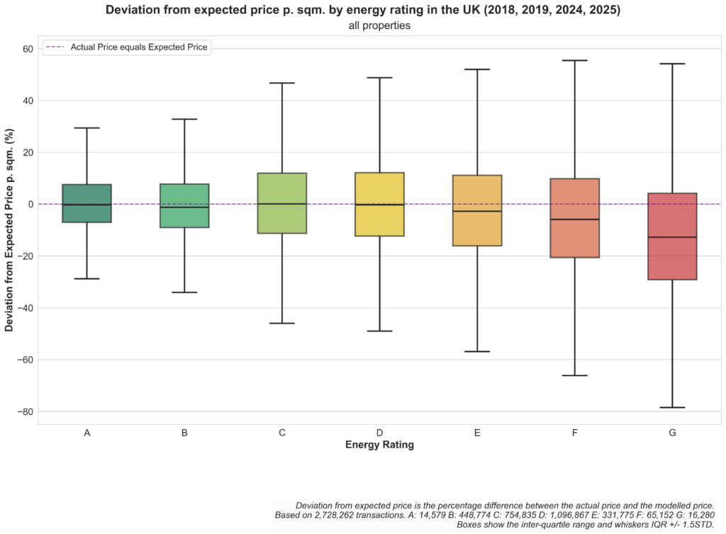
For the good energy rating classes (A-C) there is no perceivable difference between the actual price paid and the expected price.
For the poor energy rating classes (E-G) the actual price tends to be lower than the expected price. The worse the energy rating, the bigger the price difference.
The main finding is that a good energy rating has little effect on property prices, but a poor-one can negatively affect the price. The high variance in the data does however suggest that the question is more nuances and those nuances may not be captured in this high-level analysis. A more detailed analysis is needed to get a clearer picture about the complicated relationship between energy performance and property pricing.
We provide a more detailed description of our analysis below where we discuss among other things, data acquisition, join, cleaning, regression model features, regression analysis and analysis of EPC pricing over time, property type and location.
Custom urban data analysis
This story is provides high level insights drawn from the analysis of one or more open source urban data-sets. In case you find this story interesting, please contact us for more information as well as pricing and availability of a custom urban data analysis.
Full Report
Data Acquisition
We download the data for Price Paid (PP) and Energy Performance Certificates (EPC) from HM Land Registry and Ministry of Housing, Communities and Local Government, respectively. The Price Paid data can be downloaded for each year separately. The Energy Performance Certificates can be downloaded as a single file and it contains full history of certificates.
After looking briefly at the yearly transaction volume and price volatility over the years, we noticed a drop in property transactions during the COVID pandemic of 2020 and 2021. In order to focus on the impact of Energy Performance Ratings we wanted other parts of the market to be as stable as possible. Hence we decided to leave out the two disrupted year as well as 2022, in order to allow the market to stabilize before entering our analysis.
Dataset Join
Although the UK has a unique property reference number system, this information is not available in the Price-Paid dataset. Therefore we need to join the datasets based on the postal address of the properties.
In order to handle inconsistent writing of addresses we apply a combination of exact address match, an address rewrite heuristic and a proprietary machine learned address rewrite model.
Properties can have multiple records in both the PP dataset and the EPC dataset since each property can be either sold or assessed at different times. We join each record in the PP dataset with the latest energy performance certificate generated before the property transaction.
Using our hybrid data join approach, we were able to join 91.6% of the price-paid transactions to a corresponding entry in the EPC dataset.
Data Cleaning
We clean the PP dataset by:
- Eliminating properties of type “other”
- Restricting transactions to Standard Price Paid transactions
- Eliminating properties with a missing postcode
We clean the EPC dataset by:
- Eliminating properties with zero floor area
- Eliminating properties with a missing postcode
We further remove outliers where the price per m2 falls outside the interquartile range with k = 1.5. The price outliers are calculated for each postcode area and year separately in order to minimize the effect of geographic and temporal price changes.
We also eliminated large properties from our data set, i.e. properties with either 10 or more habitable rooms or a total floor area of 500 m2.
Regression Model Features
In order to create a regression model for predicting the expected price per m2 of residential properties we generate a set of features with different characteristics.
Property type
We generate four boolean features for property types.
- Property type (detached)
- Property type (flats and maisonettes)
- Property type (semi-detached)
- Property type (terraced)
Land ownership
We calculate one boolean feature for representing the two possible cases whether the land is sold together with the property (freehold) or if the property is on leased land (leasehold).
- Freehold vs leasehold
Property age
We calculate four boolean features based on the age band of the property and one boolean feature representing whether the property is a new-build or an existing property.
- Age-band (before-1900)
- Age-band (1900-1949)
- Age-band (1950-1999)
- Age-band (2000-2049)
- New-build vs existing
Property characteristics
We include multiple boolean features to represent the number of habitable rooms, total floor area, and floor level.
- Habitable rooms: 1
- Habitable rooms: 2-3
- Habitable rooms: 4-5
- Habitable rooms: 6-9
- Habitable rooms: 10+ (eliminated in data cleaning, see above)
- Floor-area: 0-50 m2
- Floor-area: 50-70 m2
- Floor-area: 70-100 m2
- Floor-area: 100-150 m2
- Floor-area: 150+ m2
- Floor-level: bottom
- Floor-level: top
Property tenure
We include three features based on the tenure of the property.
- Tenure: owner occupied
- Tenure: private rental
- Tenure: social rental
Historic property prices
We calculate multiple features based on historic property prices of “comparable properties” in a the surrounding geographic area. All prices are converted into price per m2. We aggregate prices both with and without taking the property type into account. We seek to find the right balance between meaningful statistic and geographic specificity. We only calculate price averages if 10 or more comparable properties are found. We traverse the geographic hierarchy from postcode to postcode sector to postcode district to postcode area. For a given property transaction, if less that 10 comparable property transactions exist for the preceding time period and within the same postcode as the given property, we proceed to the postcode sector level, if we again fail to find at least 10 transactions at the postcode sector level we move to the postcode district level, etc. We calculate historic prices over three temporal periods, previous month, quarter and year.
The resulting list of historic property price features are as follows:
- Previous year price p. m2 (same property type)
- Previous year price p. m2
- Previous quarter price p. m2 (same property type)
- Previous quarter price p. m2
- Previous month price p. m2 (same property type)
- Previous month price p. m2
Transaction counts
We calculate four features based on historic transaction counts in the vicinity of the property sold.
- Previous year transaction count (postcode)
- Previous year transaction count (postcode sector)
- Previous year transaction count (postcode district)
- Previous year transaction count (postcode area)
Regression Analysis
In order to get a feel for how useful different features are to model the expected property price p. m2, we perform a regression analysis using both individual features and combination of features.
We start with evaluating each feature individually and measure how much of the variance in the depended variable (property price p. m2) can be explained by that feature. In the analysis below, that value is reported as Individual R2.
We then order the feature-set by the Individual R2 and evaluate a series of models of 1 to k features, where we incrementally add the features. The outcome of that model is reported as Total R2. In this setup we also evaluate the impact of incrementally adding a feature and call it Incremental R2.
We carry this analysis out for residential property sales over 4 years, 2018, 2019, 2024 and 2025. The data represents two years before and two years after the COVID pandemic.
The results of the regression analysis be seen in the table below. The analysis is based on a set of 2,728,262 residential property transactions.
We see that Price History features are the most effective features for explaining the variance in the dependent variable, each with an Individual R2 value between 75% and 80%.
Looking at the Incremental and Total R2 values we see that after adding the first of those price history features, the average local price per m2 during the previous year, the following price history features have a limited impact on pushing up the Total R2 value (1.33 percentage points).
The remaining features also have limited impact, pushing the Total R2 up by 2.37 percentage points to 84.08%.
_Property type (flats and maisonettes)_ is the best performing non-price-history feature, with and Individual R2 score of 6.08%. However, when added incrementally after the price-history features, its impact is negligible (0.06 percentage points).
The same is the case for most other features, although the floor area features seem to be able to add useful nuances to the model when added incrementally (1.76 percentage points).
| name | Individual R2 | Incremental R2 | Total R2 |
|---|---|---|---|
| Prev. year price p. m2 (same prop. type) | 80.38% | 80.38% | 80.38% |
| Prev. year price p. m2 | 79.40% | 0.66% | 81.04% |
| Prev. quarter price p. m2 (same prop. type) | 77.84% | 0.37% | 81.41% |
| Prev. quarter price p. m2 | 77.65% | 0.01% | 81.42% |
| Prev. month price p. m2 (same prop. type) | 75.34% | 0.29% | 81.71% |
| Prev. month price p. m2 | 74.90% | 0.00% | 81.71% |
| Property type (flats and maisonettes) | 6.08% | 0.06% | 81.77% |
| Prev. year transaction count (postcode area) | 4.62% | 0.00% | 81.77% |
| Freehold vs leasehold | 2.40% | 0.03% | 81.80% |
| Habitable rooms: 4-5 | 1.84% | 0.02% | 81.82% |
| Floor-area: 0-50 m2 | 1.75% | 0.36% | 82.17% |
| Property type (terraced) | 1.28% | 0.05% | 82.22% |
| Floor-area: 70-100 m2 | 1.04% | 0.00% | 82.22% |
| Habitable rooms: 2-3 | 0.97% | 0.03% | 82.25% |
| Floor-level: bottom | 0.95% | 0.00% | 82.25% |
| Property type (semi-detached) | 0.87% | 0.02% | 82.27% |
| Floor-level: top | 0.54% | 0.04% | 82.32% |
| Prev. year transaction count (postcode district) | 0.45% | 0.00% | 82.32% |
| New-build vs existing | 0.35% | 0.25% | 82.57% |
| Prev. year transaction count (postcode sector) | 0.35% | 0.00% | 82.57% |
| Tenure: owner occupied | 0.29% | 0.00% | 82.57% |
| Habitable rooms: 1 | 0.25% | 0.00% | 82.57% |
| Floor-area: 50-70 m2 | 0.24% | 1.29% | 83.86% |
| Age-band (1950-1999) | 0.14% | 0.05% | 83.91% |
| Floor-area: 150+ m2 | 0.11% | 0.11% | 84.02% |
| Floor-area: 100-150 m2 | 0.05% | 0.00% | 84.02% |
| Property type (detached) | 0.02% | 0.00% | 84.02% |
| Tenure: private rental | 0.02% | 0.02% | 84.04% |
| Age-band (2000-2049) | 0.01% | 0.00% | 84.04% |
| Prev. year transaction count (postcode) | 0.01% | 0.00% | 84.04% |
| Age-band (1900-1949) | 0.00% | 0.01% | 84.05% |
| Tenure: social rental | 0.00% | 0.02% | 84.07% |
| Habitable rooms: 6-9 | 0.00% | 0.00% | 84.08% |
| Age-band (before-1900) | 0.00% | 0.00% | 84.08% |
In order to view at the impact of Energy Performance Rating on Property Price from a regression analysis viewpoint we continue the the same analysis process using a number of features based on the Energy Performance Rating of properties (see table below). Looking at the Incremental R2 we see that the energy performance rating can only explain a few percentage points of the overall variance when other features have been accounted for.
| name | Individual R2 | Incremental R2 | Total R2 |
|---|---|---|---|
| Energy Performance Rating (ABC) | 0.53% | 0.00% | 84.08% |
| Energy Performance Rating (EFG) | 0.38% | 0.02% | 84.10% |
| Energy Performance Rating (AB) | 0.46% | 0.01% | 84.11% |
| Energy Performance Rating (FG) | 0.19% | 0.01% | 84.12% |
| Energy Performance Rating (A) | 0.02% | 0.00% | 84.12% |
| Energy Performance Rating (B) | 0.44% | 0.00% | 84.12% |
| Energy Performance Rating (C) | 0.06% | 0.00% | 84.12% |
| Energy Performance Rating (D) | 0.08% | 0.00% | 84.12% |
| Energy Performance Rating (E) | 0.20% | 0.00% | 84.12% |
| Energy Performance Rating (F) | 0.12% | 0.00% | 84.12% |
| Energy Performance Rating (G) | 0.07% | 0.00% | 84.12% |
Note that the Energy Performance Rating results are only presented here for informative purposes and those features are not included in our final model.
Pricing of Energy Performance Certificates
In order to investigate whether ECP rating has an impact on the pricing of residential properties we use the linear regression model developed in the previous section to predict an expected price for each property and then calculate a new value representing the difference in the modeled (expected) price and the actual price. I.e., we take the modeled price as the expected price and look at how the actual price deviated from the expected price. Positive values mean that the actual price was higher than the expected price.
The figure below shows an overview of the price deviation for all properties sold in the UK in 2018, 2019, 2024 and 2025.
For the good energy rating classes (A-C) there is no perceivable difference between the actual price and the expected price.
For the poor energy rating classes (E-G) the actual price is on average lower than the expected price. The worse the energy rating, the bigger the price difference.
The main finding is that a good energy rating has little effect on property prices, but a poor-one can negatively affect the price. The high variance in the data does however suggest that the question is more nuances and those nuances may not be captured in this high-level analysis. A more detailed analysis is needed to get a clearer picture about the complicated relationship between energy performance and property pricing. We will not go into all the details in this post but look briefly at three aspects: time, property type and location.
Pricing Over Time
The figure below shows the price deviation for each Energy Performance Rating and each year separately.
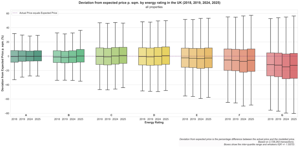
We see that the overall price deviation for poor energy performance is quite stable between years. There are some minor price change pattern between years, but it seems to be equal across all energy performance ratings and more likely to be due to our model not capturing fully the effect of changing house price index over time.
Pricing Over Property Types
Below we see a series of price deviation plots for different property types.
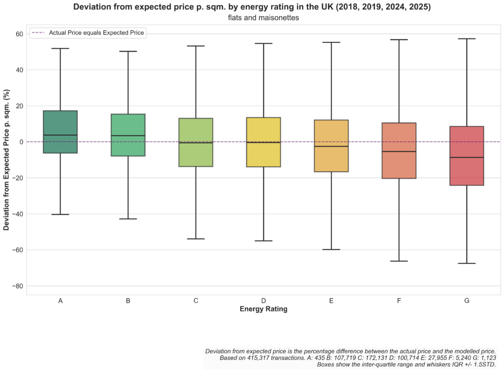
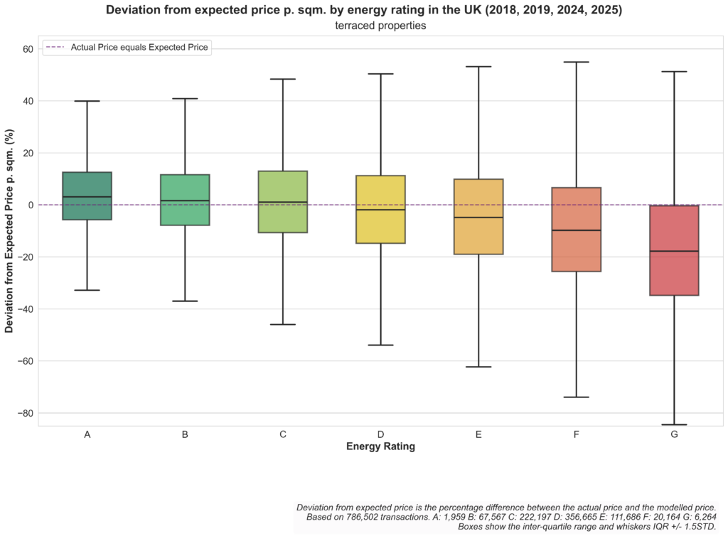
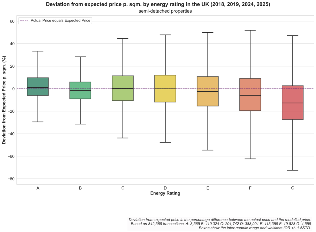
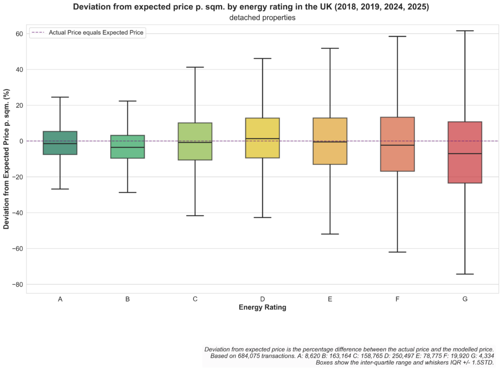
There are some differences between property types. For Flats and maisonettes and Terraced properties with energy performance rating A the actual price is more often than not slightly higher than the expected price. Whereas the price deviation for Detached properties is more even over all energy performance ratings.
Pricing Over Location
In order to demonstrate how the results can change from one location to another we look at two example locations. Bradford (postcode area BD) is one of the postcode areas with the highest variance in price deviation across energy performance ratings and Kingston upon Thames (postcode area KT) is on the other hand one of the postcode areas with the lowest variance in price deviation across different rating classes.
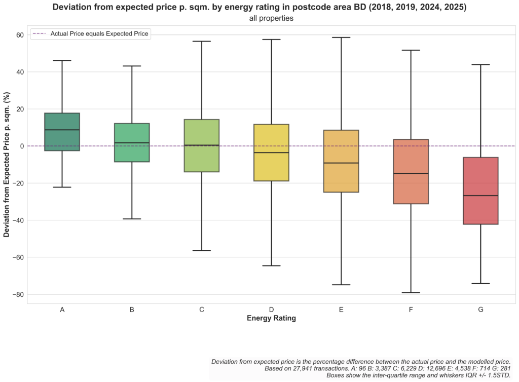
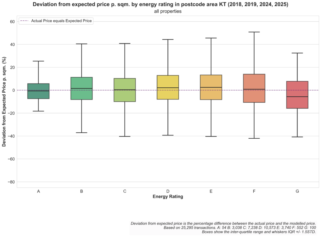
We have not gone into depth to try to explain why the energy performance rating may affect property prices in different ways in different locations, but a quick look reveals that the three postcode areas with the highest variance across EPC classes (Bradford (BD), Blackburn (BB) and Wakefield (WF)) are among the more deprived area in the UK and the three postcode areas with the lowest variance (Chelmsford (CM), Redhill (RH) and Kingston upon Thames (KT) are among the less deprived areas. These are just anecdotal observations that could be worth a deeper analysis.
Discussion
This analysis of the pricing of Energy Performance Certificates in the UK only scratches the surface of a complex topic. We addressed it with the very generic question in mind, i.e. to see if the energy performance certificates had any impact at all on the pricing of residential properties.
We found that the answer to the question is quite nuanced and it depends on many factors, including property type and location. And the location parameter might be a proxy for other underlying parameters such as demographics and/or housing stock.
For the price modeling in this study we chose linear regression due to its simplicity and suitability for looking into the impact of different independent variables. There is no doubt scope for exploring the application of a more sophisticated modeling approach.
Custom urban data analysis
This story is provides high level insights drawn from the analysis of one or more open source urban data-sets. In case you find this story interesting, please contact us for more information as well as pricing and availability of a custom urban data analysis.